1. introduction
In this blog, I will present one of my foundational projects – a Bank Customer Churn Prediction using a classification approach. This project falls into the same category as the customer credit classification prediction I mentioned in a previous blog post. However, the focus is distinct. In my prior professional risk analyst job experiences, the most challenging aspects revolved around data collection and processing. Nonetheless, in this current project, the data was obtained from Kaggle and is structured in nature. This aspect significantly mitigated the data-related challenges. Consequently, the primary emphasis of this project lies in utilizing fundamental machine learning models for classifying and predicting outcomes on a small-scale dataset. The specific code implementation will be provided in the appendix of this blog post.
This project is primarily divided into three major sections: Part 1: Data Exploration, Part 2: Feature Preprocessing, and Part 3: Model Training and Results Evaluation. I will also center my discussion around these three segments, along with sharing my personal insights into this project.
2. Data Exploration
In the initial phase, I delved into exploring the dataset. This involved a comprehensive analysis of the provided data to gain insights into its structure, distributions, and potential patterns. By visualizing key features and statistical summaries, I was able to identify any outliers or missing values that might affect the subsequent analysis. Additionally, I examined the distribution of the target variable – churn prediction – to understand the class distribution and potential class imbalance issues.
2.1 Understand the Raw Dataset and Features
This section is relatively straightforward, primarily involving a foundational understanding of the data. It’s a total of 10,000 data entries, and the dataset appears to be remarkably complete without any instances of missing values. Furthermore, the features encompass both numerical and categorical data types.
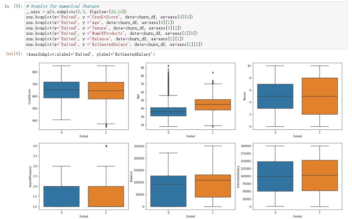
In the box plots, we can see that the “age” and “NumOfProducts” features have data points that extend beyond the typical range. However, it’s essential not to immediately classify these data points as outliers. Further investigation during the feature engineering phase is warranted to thoroughly analyze these features.
3. Feature Preprocessing
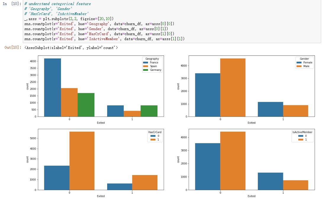
Feature preprocessing played a pivotal role in this project. This phase encompassed various steps, including data cleaning, encoding categorical variables, and scaling numerical features. Dealing with categorical variables involved techniques such as one-hot encoding or label encoding, depending on the nature of the data. I also performed feature scaling to ensure that numerical features were on a comparable scale, which is vital for many machine learning algorithms. I using box plots and histograms to provide valuable insights into numerical and categorical data respectively.
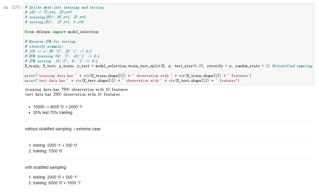
3.1 Split dataset
I began categorizing the data into two main types: descriptive data and numerical data. This initial step was crucial in acknowledging the distinct nature of these data types and laying the groundwork for tailored preprocessing techniques. Following this classification, I moved on to a pivotal step in any machine learning endeavor – data splitting. This involved partitioning the dataset into two subsets: training data and testing data.
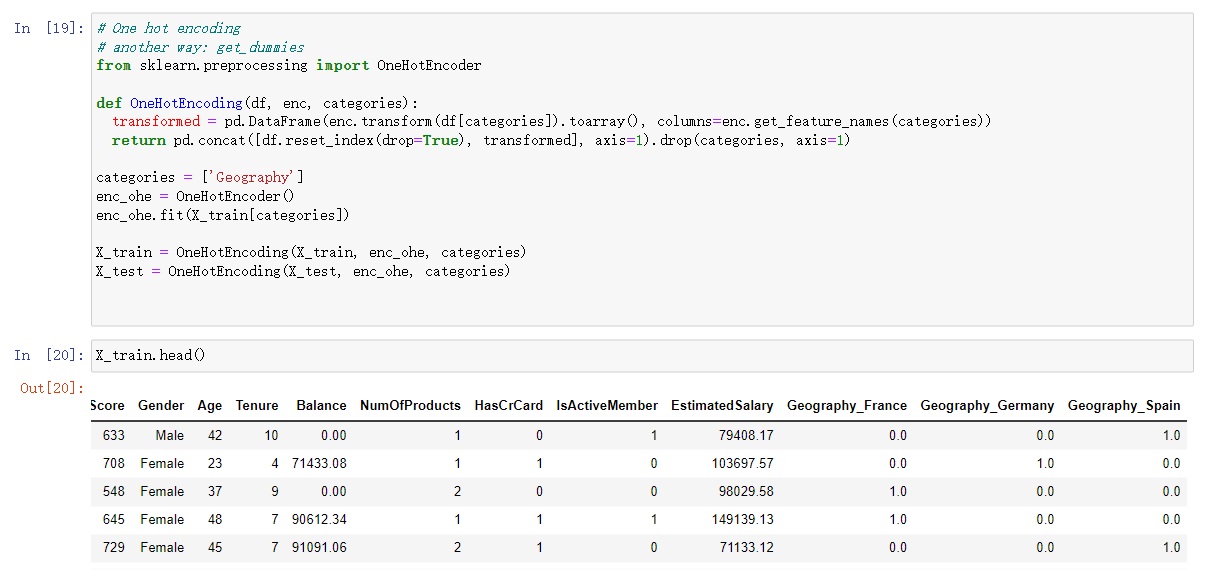
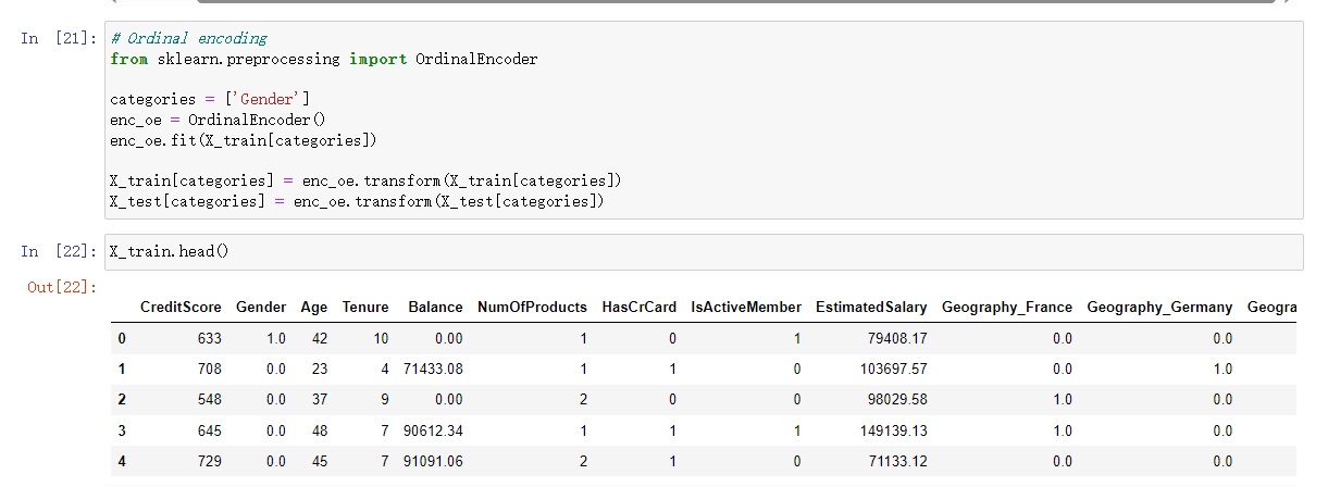
3.2 Encoding
Two categorical features, “Geography” and “Gender,” required specific treatment. For “Geography,” I employed the one-hot encoding technique. This method transformed the categorical labels into binary columns, allowing the model to comprehend the categorical information effectively.
In the case of “Gender,” I opted for ordinal encoding. This approach assigned numerical values to the categories, preserving the order while steering clear of creating an excessive number of new columns.
3.3 Standardization
At last of this part, I need to standardizing these data. This process is an essential preprocessing technique that transforms the numerical features to have a mean of 0 and a standard deviation of 1. By doing so, the data is brought onto a common scale, preventing any single feature from disproportionately influencing the model’s behavior.
4. Model Training and Results Evaluation
The final phase focused on model training and evaluation. I experimented with fundamental machine learning models like logistic regression, decision trees, and random forests due to the relatively small size of the dataset. The models were trained on a portion of the data and validated on another portion to assess their performance. Key metrics such as accuracy, precision, recall, and F1-score were used to evaluate the models. I also implemented techniques like cross-validation and hyperparameter tuning to enhance the model’s performance.
4.1 Model Training
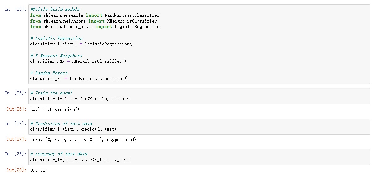
In this phase, I ventured into the heart of the project – training and evaluating machine learning models. Considering the moderate dataset size and the need for both accuracy and interpretability, I carefully selected three distinct models: Logistic Regression, K Nearest Neighbors (KNN), and Random Forest.
4.2 Use Grid Search to Find Optimal Hyperparameters
As we delve deeper into this project, a pivotal phase emerges – the fine-tuning of our models for peak performance. To accomplish this, I harnessed the power of grid search, a technique that systematically explores a range of hyperparameter values to unearth the optimal combination.
Logistic Regression: For this model, I meticulously fine-tuned hyperparameters such as the regularization strength (C), which controls the trade-off between fitting the training data and preventing overfitting. By utilizing grid search, I aimed to identify the ideal C value that strikes the perfect balance.
K Nearest Neighbors (KNN): The number of neighbors (k) is a key hyperparameter in KNN. Through grid search, I sought to determine the optimal k value that would lead to the best model performance. This iterative process allowed me to make informed decisions about the number of neighbors to consider for classification.
Random Forest: In the realm of Random Forest, the number of trees and the depth of each tree are critical hyperparameters. Grid search helped me pinpoint the combination that maximized the model’s predictive capabilities. This optimization ensures that the Random Forest leverages the strengths of its individual trees while avoiding overfitting.
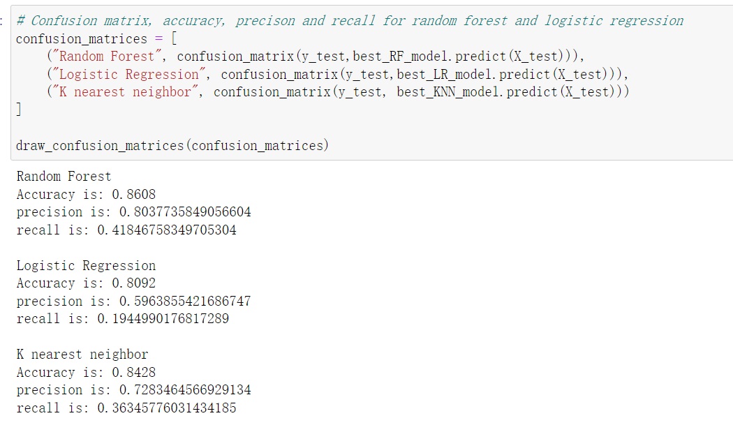
4.3: Model Evaluation - Confusion Matrix (Precision, Recall, Accuracy)
In this part, I will using the confusion matrices to analyse our fine-tuned models – Logistic Regression, KNN, and Random Forest – I gained an in-depth understanding of their strengths and weaknesses. This exploration allowed me to make informed decisions about the models’ predictive abilities, identify potential areas of improvement, and choose the one that aligns best with the project’s objectives.
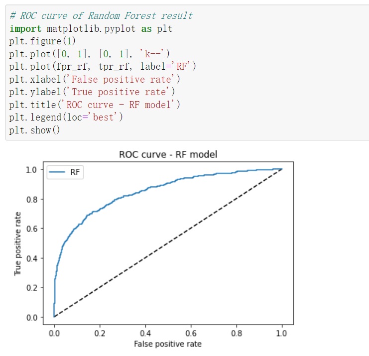
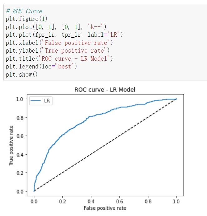
4.4 Model Evaluation - ROC & AUC
By plotting the ROC curves and calculating the AUC scores for our optimized models – Logistic Regressionand Random Forest – I will get the capabilities across different classification thresholds. This visual and numerical insight provided a deeper understanding of their strengths and helped in making the final decision on the model selection.
4.5 Feature Importance Discussion
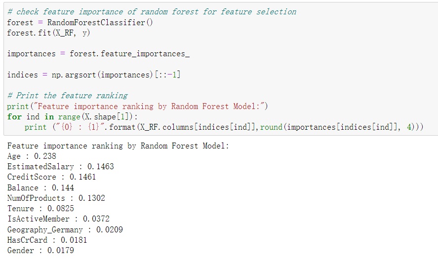
The feature Importance is A pivotal aspect of Random Forest lies in its ability to assign importance scores to each feature. These scores illuminate which attributes contribute most to the model’s decision-making process. By delving into these scores, we can pinpoint the features that play a crucial role in predicting customer churn.
In the grand finale of this project, I explored the feature importance scores and uncovered the top influencers on the model’s predictions. The findings highlighted that Age, EstimatedSalary, and CreditScore were the primary drivers impacting the model’s performance. This insight can be invaluable for decision-makers seeking to understand the underlying factors contributing to customer churn.
Conclution
As I wrap up this project and reflect on the journey from inception to completion, I am reminded of the intricate and rewarding nature of machine learning. The endeavor to predict bank customer churn has been an enlightening experience, showcasing the power of data-driven decision-making.
From the initial stages of data exploration and preprocessing to the meticulous model selection and evaluation, every step brought new insights and challenges. The project’s focus on interpreting results and balancing accuracy with interpretability underscored the delicate dance between complexity and simplicity in the world of machine learning.
As I bring this project to a close, I’m excited to share the final model selection, consolidate the key takeaways, and express my gratitude for the opportunity to delve into the exciting world of predictive modeling.
Project Link: https://github.com/lepingqian/Bank_Customer_Churn_Prediction